21. Multiple Integrals in Curvilinear Coordinates
e. Integrating in 3D Curvilinear Coordinates
1. Grid Cells
Now we are going to look at curvilinear coordinates in 3D, which will be similar to their 2D counterparts. As you read, you should look back at the 2D derivation to see the parallels and for details about certain quantities, such as the definition of the tangent vectors, e.g. \(\vec{e}_u\), and of their stretched versions, e.g. \(\vec{U}\).
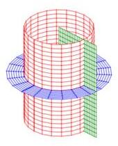
Cylindrical and spherical coordinates are the most common curvilinear coordinate system in 3D, but there are others. Several of their coordinate surfaces are shown below.
We know how to integrate in cylindrical and spherical coordinates. We would like to know how to integrate in other 3D coordinate systems as well. In the section on spherical coordinates, you were told the differential of volume was \(dV=\rho^2\sin\phi\,d\rho\,d\theta\,d\phi\) but this was not derived. Now as we discuss general curvilinear coordinates, we will use spherical coordinates as a concerete example and in the process derive the spherical differential of volume.
Coordinate System
To specify a coordinate system, we need to give the position \((x,y,z)\) as a function of the curvilinear coordinates.
Spherical coordinates are given in components by \[ x=\rho\sin\phi\cos\theta\qquad y=\rho\sin\phi\sin\theta\qquad z=\rho\cos\phi \] or as a single vector equation for the position: \[ (x,y,z)=\vec{R}(\rho,\phi,\theta) =\left\langle \rho\sin\phi\cos\theta,\rho\sin\phi\sin\theta,\rho\cos\phi\right\rangle \] Once we specify the values of \(\rho\), \(\phi\) and \(\theta\), we know the rectangular coordinates \(x\), \(y\) and \(z\).
General curvilinear coordinates are given in components by: \[ x=x(u,v,w) \qquad y=y(u,v,w) \qquad z=z(u,v,w) \] or as a single vector equation for the position: \[ (x,y,z)=\vec{R}(u,v,w) =\left\langle x(u,v,w),y(u,v,w),z(u,v,w) \right\rangle \] Once we specify the values of \(u\), \(v\) and \(w\), we know the rectangular coordinates \(x\), \(y\) and \(z\).
Coordinate Grid and Coordinate Curves
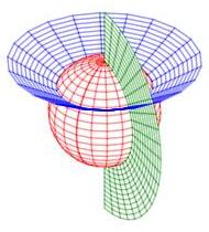
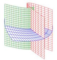
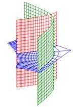
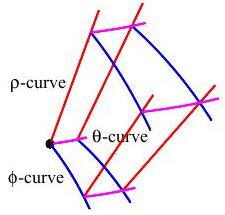
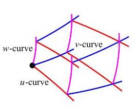
Here is the spherical coordinate grid (again) and a general 3D curvilinear coordinate grid:
There are three families of coordinate curves that define the edges of the grid cells (or coordinate boxes).
In spherical coordinates, the radial lines
(red) are called \(\rho\)-curves
because \(\rho\) is changing, the circles of longitude
(blue) are called \(\phi\)-curves
because \(\phi\) is changing and the circles of latitude
(magenta) are called \(\theta\)-curves
because \(\theta\) is changing.
The \(\rho\)-curve with \(\phi=\phi_0\) and \(\theta=\theta_0\) is
\(\vec{R}(\rho,\phi_0,\theta_0)
=\left\langle \rho\sin\phi_0\cos\theta_0,\rho\sin\phi_0\sin\theta_0,
\rho\cos\phi_0\right\rangle\)
with \(\rho\) as the parameter.
The \(\phi\)-curve with \(\rho=\rho_0\) and \(\theta=\theta_0\) is
\(\vec{R}(\rho_0,\phi,\theta_0)
=\left\langle \rho_0\sin\phi\cos\theta_0,\rho_0\sin\phi\sin\theta_0,
\rho_0\cos\phi\right\rangle\)
with \(\phi\) as the parameter.
The \(\theta\)-curve with \(\rho=\rho_0\) and \(\phi=\phi_0\) is
\(\vec{R}(\rho_0,\phi_0,\theta)
=\left\langle \rho_0\sin\phi_0\cos\theta,\rho_0\sin\phi_0\sin\theta,
\rho_0\cos\phi_0\right\rangle\)
with \(\theta\) as the parameter.
In the general curvilinear coordinates, there are \(u\)-curves
(red) on which \(u\) is changing,
\(v\)-curves (blue) on which \(v\)
is changing, and \(w\)-curves (magenta)
on which \(w\) is changing.
The \(u\)-curve with \(v=v_0\) and \(w=w_0\) is
\(\vec{R}(u,v_0,w_0)
=\left\langle x(u,v_0,w_0),y(u,v_0,w_0),z(u,v_0,w_0) \right\rangle\)
with \(u\) as the parameter.
The \(v\)-curve with \(u=u_0\) and \(w=w_0\) is
\(\vec{R}(u_0,v,w_0)
=\left\langle x(u_0,v,w_0),y(u_0,v,w_0),z(u_0,v,w_0) \right\rangle\)
with \(v\) as the parameter.
The\(w\)-curve with \(u=u_0\) and \(v=v_0\) is
\(\vec{R}(u_0,v_0,w)
=\left\langle x(u_0,v_0,w),y(u_0,v_0,w),z(u_0,v_0,w) \right\rangle\)
with \(v\) as the parameter.
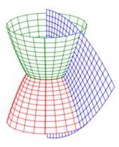
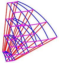
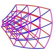
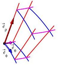
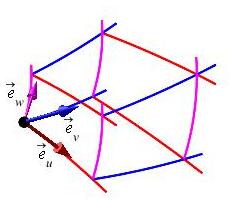
Since the grid is so crowded, we concentrate on one grid cell:
Coordinate Tangent Vectors
The tangent vector to a parametric curve, \(\vec r(t)\), is the derivative of the position with respect to its parameter: \[ \vec e_t=\dfrac{d\vec r}{dt} =\left\langle \dfrac{dx}{dt},\dfrac{dy}{dt},\dfrac{dz}{dt}\right\rangle \]
When dealing with a curvilinear coordinate system, the tangent vector along each coordinate curve is found by differentiating with respect to its parameter. Since the other coordinates are held fixed, these are partial derivatives.
In spherical coordinates: \[ \vec{R}(\rho,\phi,\theta) =\left\langle \rho\sin\phi\cos\theta,\rho\sin\phi\sin\theta, \rho\cos\phi\right\rangle \] The tangent vectors to the \(\rho\), \(\phi\) and \(\theta\) curves are the partial derivatives with respect to those parameters: \[\begin{aligned} \vec{e}_\rho=\dfrac{\partial\vec{R}}{\partial\rho} &=\left\langle \dfrac{\partial x}{\partial\rho}, \dfrac{\partial y}{\partial\rho},\dfrac{\partial z}{\partial\rho}\right\rangle \\ &=\left\langle \sin\phi\cos\theta,\sin\phi\sin\theta, \cos\phi\right\rangle \\ \vec{e}_\phi=\dfrac{\partial\vec{R}}{\partial\phi} &=\left\langle \dfrac{\partial x}{\partial\phi}, \dfrac{\partial y}{\partial\phi},\dfrac{\partial z}{\partial\phi}\right\rangle \\ &=\left\langle \rho\cos\phi\cos\theta,\rho\cos\phi\sin\theta, -\rho\sin\phi\right\rangle \\ \vec{e}_\theta=\dfrac{\partial\vec{R}}{\partial\theta} &=\left\langle \dfrac{\partial x}{\partial\theta}, \dfrac{\partial y}{\partial\theta},\dfrac{\partial z}{\partial\theta}\right\rangle \\ &=\left\langle -\rho\sin\phi\sin\theta,\rho\sin\phi\cos\theta, 0\right\rangle \end{aligned}\]
For general curvilinear coordinates, the coordinate tangent vectors, are: \[\begin{aligned} \vec{e}_u&=\dfrac{\partial\vec{R}}{\partial u} =\left\langle \dfrac{\partial x}{\partial u}, \dfrac{\partial y}{\partial u},\dfrac{\partial z}{\partial u}\right\rangle \\ \vec{e}_v&=\dfrac{\partial\vec{R}}{\partial v} =\left\langle \dfrac{\partial x}{\partial v}, \dfrac{\partial y}{\partial v},\dfrac{\partial z}{\partial v}\right\rangle \\ \vec{e}_w&=\dfrac{\partial\vec{R}}{\partial w} =\left\langle \dfrac{\partial x}{\partial w}, \dfrac{\partial y}{\partial w},\dfrac{\partial z}{\partial w}\right\rangle \end{aligned}\]
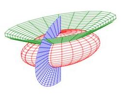
The coordinate tangent vectors are added to the coordinate grid plots below at the point \((r_0,\phi_0,\theta_0)\) for the spherical plot and at \((u_0,v_0,w_0)\) for the general curvilinear plot.
Heading
Placeholder text: Lorem ipsum Lorem ipsum Lorem ipsum Lorem ipsum Lorem ipsum Lorem ipsum Lorem ipsum Lorem ipsum Lorem ipsum Lorem ipsum Lorem ipsum Lorem ipsum Lorem ipsum Lorem ipsum Lorem ipsum Lorem ipsum Lorem ipsum Lorem ipsum Lorem ipsum Lorem ipsum Lorem ipsum Lorem ipsum Lorem ipsum Lorem ipsum Lorem ipsum